Performing Early Warning Signal Assessments

Duncan O’Brien

2024-08-27

About this tutorial

This tutorial introduces how to perform both univariate and multivariate early warning signal (EWS) assessments using EWSmethods. It will give examples of rolling and expanding window approaches for univariate data, introduce trait-based composite EWSs and then conclude with an example of multivariate EWSs.

Greater detail on each function can be found at the Reference page.

Getting started

set.seed(123) #to ensure reproducible data

library(EWSmethods)

1. The data

EWSmethods comes bundled with two data objects which allow you to practice using the uniEWS() and multiEWS() functions in both transitioning and non-transitioning data before applying it to your own use case.

"simTransComms" contains three replicate datasets of a simulated five species community that has been driven to transition by the introduction of an invasive species (following Dakos 2018). This will be our multivariate dataset when using multiEWS() although we may also use each time series in isolation in uniEWS().

"CODrecovery" contains three replicate datasets of a simulated cod ( Gadus morhua ) population that transitions from an overfished to a recovered state following the relaxation of fishing pressure. This data was first published by Clements et al. 2019. While univariate, "CODrecovery" provides extra information on the body size of cod individuals which will improve composite EWSs estimated by uniEWS().

#Load the two datasets in to the session
data("simTransComms")

data("CODrecovery")

We can visualise a community from each of these datasets using the code below:

matplot(simTransComms$community1[,3:7], type = "l", xlab = "Time", ylab = "Density",  main = "Transitioning five species community")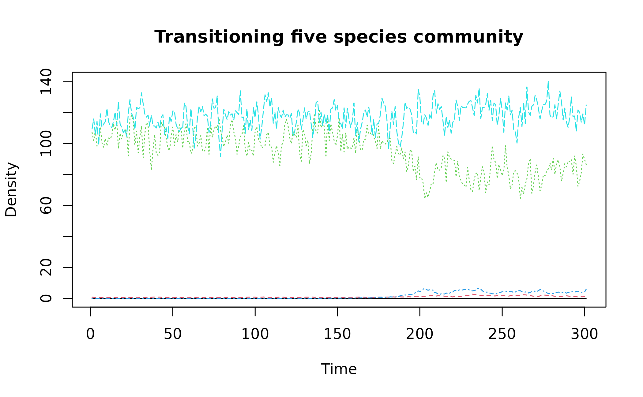

plot(x = CODrecovery$scenario2$time, y = CODrecovery$scenario2$biomass, type = "l", xlab = "Year", ylab = "Abundance", main = "Recovering cod population")

These plots show that a transition takes place at time ~= 180 in "simTransComms$community1" and year ~= 2050 in "CODrecovery$scenario2". EWSmethods helpfully provides this information in each dataset under the inflection_pt column.

simTransComms	CODrecovery
191.5	2055

However, EWS assessments are only meaningful if performed on data prior to a transition. As EWsmethods provides the time point of transition for both datasets, we can truncate our time series to pre-transition data only.

pre_simTransComms <- subset(simTransComms$community1,time < inflection_pt)

pre_CODrecovery <- subset(CODrecovery$scenario2,time < inflection_pt)

In reality, EWSs will be assessed in real-time with the presence of past/present tipping points often unknown. If past transitions are known to have occurred, it may be prudent to follow the suggestions of O’Brien & Clements (2021) who show that the occurrence of a historic transition can mask an oncoming event and that only using data post the historic transition improves EWS reliability.

Now the data has been loaded and truncated, it can now be passed to uniEWS() and multiEWS() to perform EWS assessments.

2. Univariate EWSs

EWSmethods provides two computational approaches to calculate univariate EWSs via the uniEWS() function - rolling vs expanding windows. The difference between the two is evident in the figure below but simply, rolling windows estimate EWSs in subsets of the overall time series before ‘rolling’ on one data point and reassessing, Conversely, expanding windows add data points sequentially in to an ‘expanding’ assessment and then standardises against the running mean and standard deviation of the previous window.

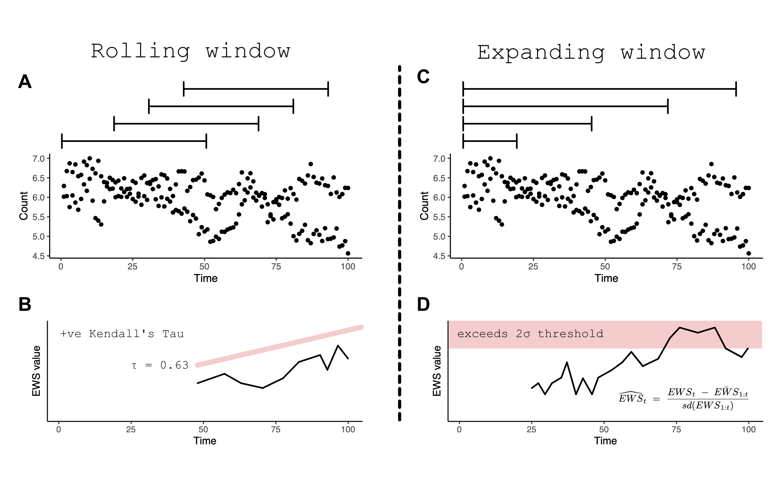
Rolling (A) vs expanding (C) window concept diagram. Panels B and D introduce the circumstance when a ‘warning’ is signalled in both approaches

Both computational approaches are able to calculate the same EWS indicators. A brief outline of each can be found in the following table as well as their reference code in uniEWS() for the metrics = argument.

EWS indicator	Description	uniEWS() metric code
Standard deviation	Increasing variance/standard deviation is observed approaching a transition	"SD"
Coefficient of variation	Equivalent to SD as is simply SD at time t divided by the mean SD of the time series	"cv"
Autocorrelation at lag1	Autocorrelation (similarity between successive observations) increases approaching a transition. The value of this indicator can be estimated as either the autocorrelation coefficient estimated from a first order autoregressive model or the estimated autocorrelation function at lag1	"ar1" - autoregressive model, "acf"- autocorrelation function
Skewness	At a transition, the distribution of values in the time series can become asymmetric	"skew"
Kurtosis	Kurtosis represents the system reaching more extreme values in the presence of a transition. Due to the increased presence of rare values in the time series, the tails of the observation distribution widen	"kurt"
Return rate	The inverse of the first-order term of a fitted autoregressive AR(1) model. Return rate is the primary quantity impacted by CSD – return rate decreases as a tipping point is approached	"rr"
Density ratio	Spectral reddening (high variance at low frequencies) occurs near transition. The density ratio quantifies the degree of reddening as the ratio of the spectral density at low frequency to the spectral density at high frequency	"dr"

Rolling windows

The rolling window approach is the most commonly used form of EWS computation due to the work of Dakos et al 2012 and the earlywarnings package. uniEWS() accepts a method = and a winsize = argument which calls the expanding window method and creates a rolling window winsize% of the total time series length.

Lets use an example where we are interested in the autocorrelation, variance and skewness of one of the five species in pre_simTransComms. First we supply a dataframe/matrix of n x 2 dimensions (first column is an equally time sequence and the second is the abundance/biomass time series) and the EWS indicator metrics. The remaining arguments specify the form of computation, window size and plotting characteristics.

rolling_ews_eg <- uniEWS(data = pre_simTransComms[,c(2,5)],
                         metrics = c("ar1","SD","skew"),
                         method = "rolling",
                         winsize = 50)

plot(rolling_ews_eg,  y_lab = "Density")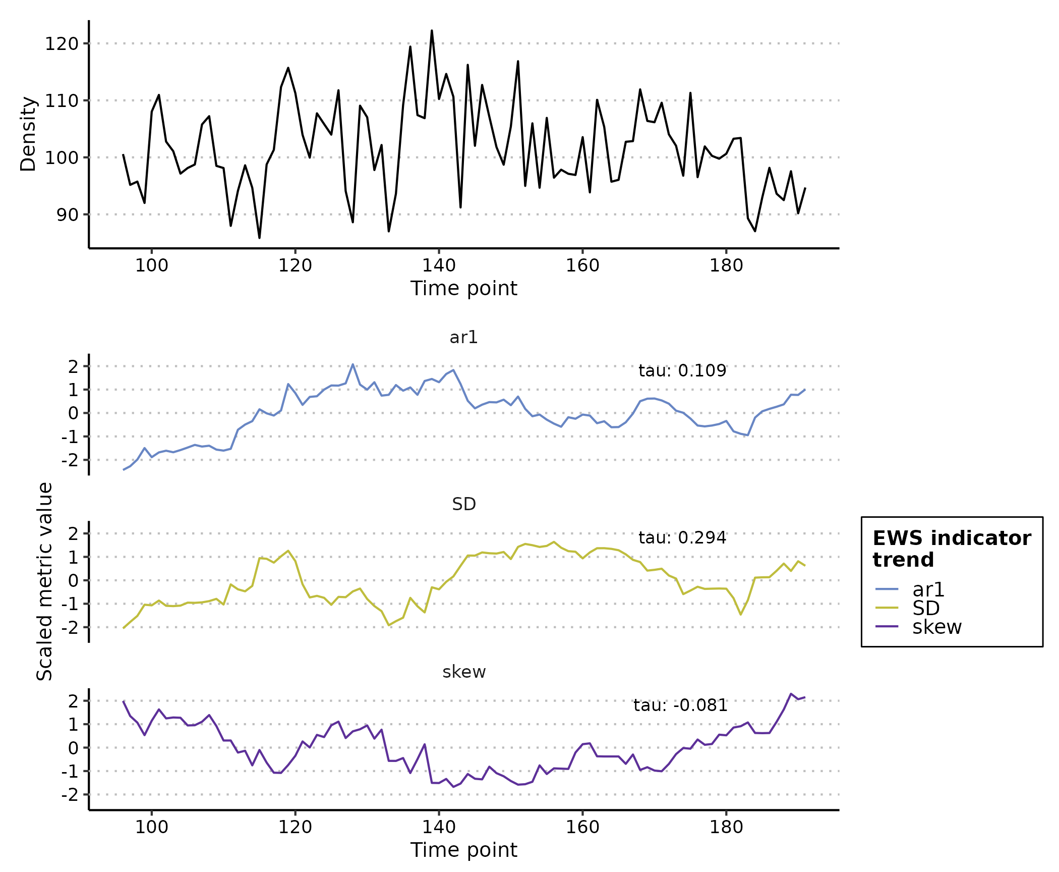

Note how all EWS indicators begin to trend upwards at time ~= 170 which results in the positive Kendall Tau correlation coefficient indicative of an oncoming transition/tipping point.

Expanding windows

Let’s explore the alternative expanding window approach. All we need to change in uniEWS() is the method = argument, and replace winsize = with burn_in =. Instead of specifying the size of the rolling window, burn_in = dictates the number of datapoints uniEWS() is to use to ‘train’ the algorithm. This mitigates the high number of false-positive signals resulting from the short time series length and high variability when few data points are supplied at the beginning of assessment (O’Brien & Clements, 2021).

expanding_ews_eg <- uniEWS(data = pre_simTransComms[,c(2,5)],
                         metrics = c("ar1","SD","skew"),
                         method = "expanding",
                         burn_in = 50,
                         threshold = 2)

plot(expanding_ews_eg, y_lab = "Density")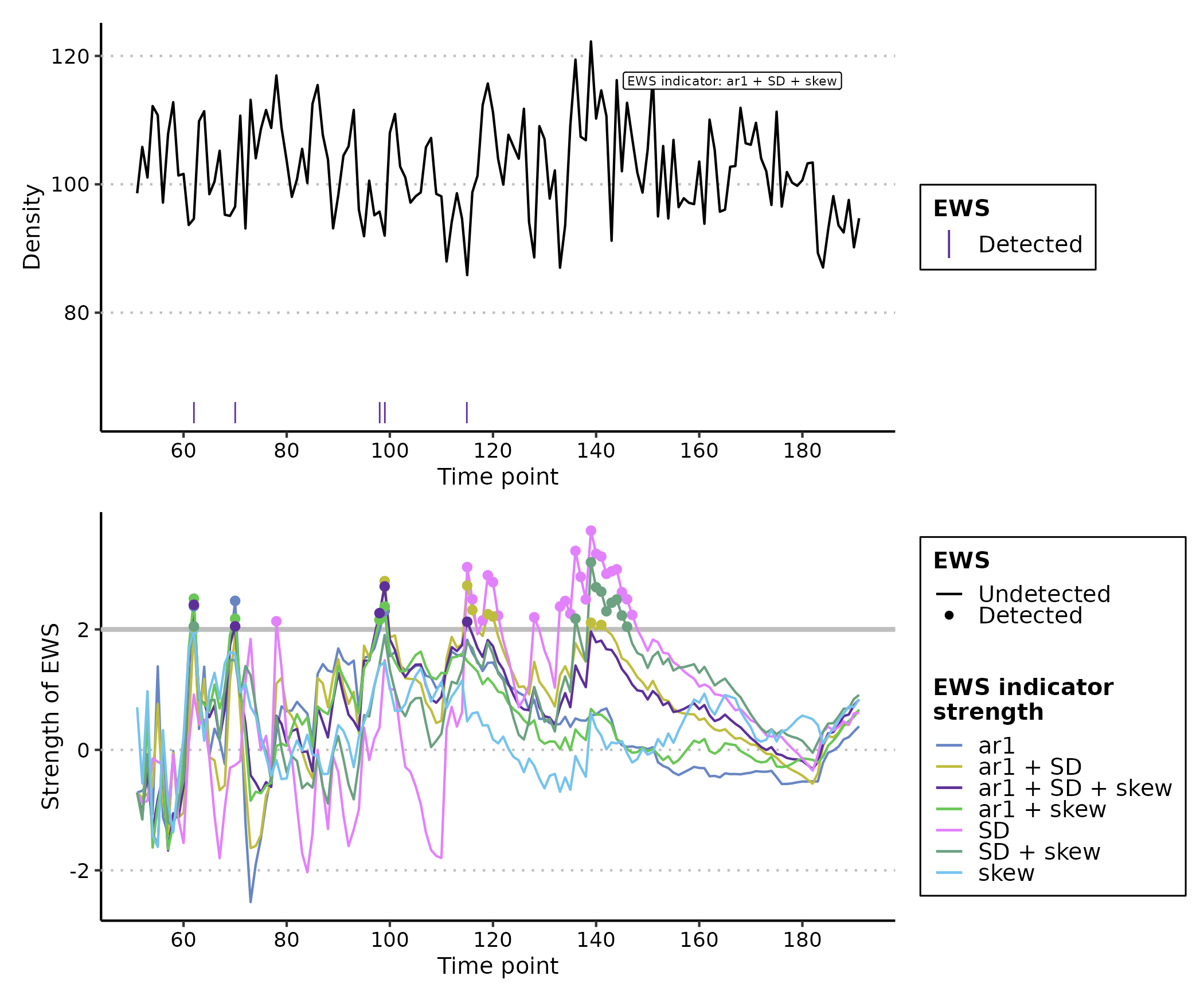

Similar to the rolling window approach, EWS indicators calculated by expanding windows have exceeded the 2σ threshold for more than two consecutive time points and thus identified warnings from time ~= 170. However we are more confident in this conclusion as the composite metrics also display this warning (ar1 + SD + skew). These composite metrics simple sum the standardised individual indicator strengths together and are known to provide a more reliable signal than lone indicators (Clements & Ozgul, 2016).

Trait information

The final contribution by uniEWS() is the ability to integrate multiple information sources in the assessment. For example, including body size estimates improves assessment reliability by reducing false positive rate whilst increasing the number of true positives (Clements and Ozgul 2016, Baruah et al. 2020). uniEWS() consequently accepts a trait = argument where an additional trait time series can be combined with the other abundance-based EWSs as a composite metric. This capability is only available if method = "expanding" and metrics = contains "trait"

trait_ews_eg <- uniEWS(data = pre_CODrecovery[,c(2,3)],
                         metrics = c("ar1","SD","trait"), #note "trait" is provided here
                         method = "expanding",
                         trait = pre_CODrecovery$mean.size, #and here
                         burn_in = 15, #small burn_in due to shorter time series
                         threshold = 2)

plot(trait_ews_eg, y_lab = "Density", trait_lab = "Mean size (g)")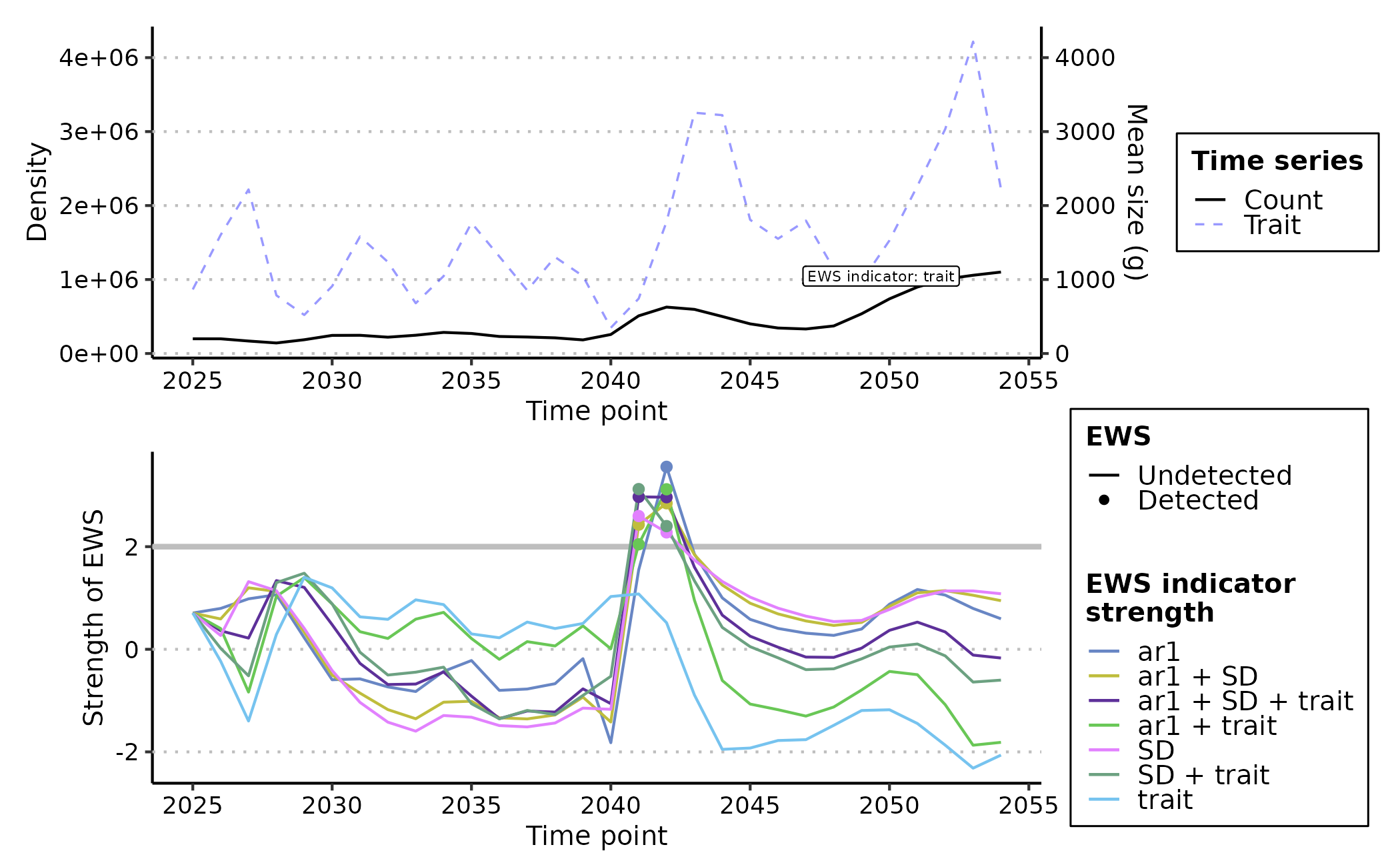

3. Multivariate EWSs

A more powerful and informative form of EWS are multivariate EWSs. These indicators combine multiple time series/measurements of the focal system to provide a community level assessment of transition risk.

There are two primary forms of multivariate EWS, those which are averaged univariate EWS across all time series and those which are assessments made on a dimension reduction of all representative time series. A brief outline of each can be found in the following table as well as their reference code in multEWS() for the metrics = argument. See Weinans et al. (2021) for a rigorous testing of these multivariate EWSs in a simulated system.

Multivariate EWS indicator	Description	multiEWS() metric code	Average or dimension reduction technique
Mean standard deviation	Average variance across all time series representing the system	"meanSD"	Average
Max standard deviation	The variance of the time series with the highest variance of all assessed time series	"maxSD"	Average
Mean autocorrelation at lag1	Average autocorrelation across all time series representing the system	"meanAR"	Average
Max autocorrelation at lag1	The autocorrelation of the time series with the highest autocorrelation of all assessed time series	"maxAR"	Average
Dominant MAF (maximum autocorrelation factor) eigenvalue	The minimum eigenvalue of the system following MAF dimension reduction	"eigenMAF"	Dimension reduction
MAF autocorrelation	The autocorrelation of the data projected on to the first MAF – i.e. the autocorrelation of the first MAF.	"mafAR"	Dimension reduction
MAF standard deviation	The variance of the data projected on to the first MAF – i.e. the variance of the first MAF	"mafSD"	Dimension reduction
First PC (principal component) autocorrelation	The autocorrelation of the data projected on to the first PC – i.e. the autocorrelation of the first PC	"pcaAR"	Dimension reduction
First PC standard deviation/ Explained variance	The variance of the data projected on to the first PC – i.e. the variance of the first PC	"pcaSD"	Dimension reduction
First PC standard deviation/ Explained variance	The variance of the data projected on to the first PC – i.e. the variance of the first PC	"pcaSD"	Dimension reduction
Dominant eigenvalue of the covariance matrix	The maximum eigenvalue of the covariance matrix between all representative time series	"eigenCOV"	Neither
Maximum covariance	The maximum value of the covariance matrix between all representative time series.	"maxCOV"	Neither
Mutual information	The ‘amount of information’ one time series contains on another.	"mutINFO"	Neither

Using multiEWS() we can estimate each of these multivariate indicators in the same way as uniEWS() - specifying the method =, winsize = and/or burn_in = - but must provide a n x m dataframe/matrix of all representative time series. The first column must again be an equally spaced time sequence.

A rolling window assessment would therefore be coded as such:

multi_ews_eg <- multiEWS(data = pre_simTransComms[,2:7],
                         metrics = c("meanAR","maxAR","meanSD","maxSD","eigenMAF","mafAR","mafSD","pcaAR","pcaSD","eigenCOV","maxCOV","mutINFO"),
                         method = "rolling",
                         winsize = 50)

plot(multi_ews_eg)

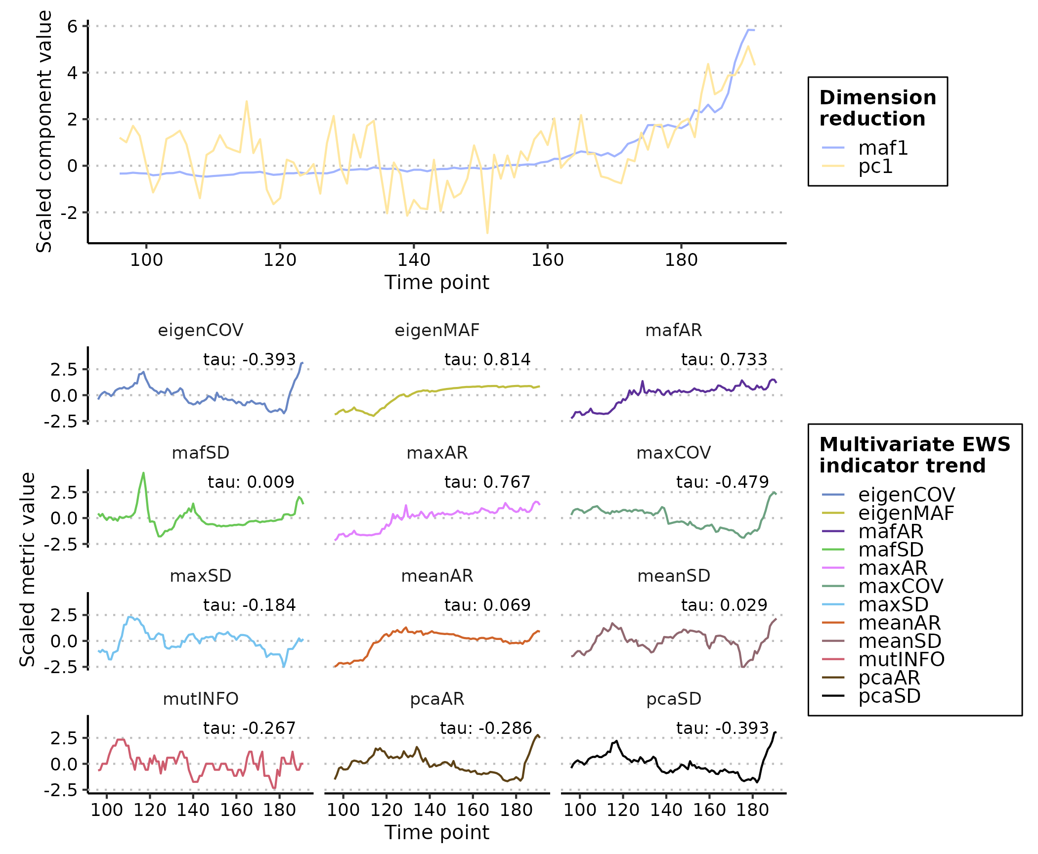
Many of these indicators are postively correlated with time and therefore are ‘warnings’.

We could also use expanding windows to achieve a similar result. Note - no composite metric is computed in multiEWS() as it is currently unknown how combining multivariate EWS indicators influences prediction reliability.

multi_ews_eg2 <- multiEWS(data = pre_simTransComms[,2:7],
                         method = "expanding",
                         burn_in = 50,
                         threshold = 2)

plot(multi_ews_eg2)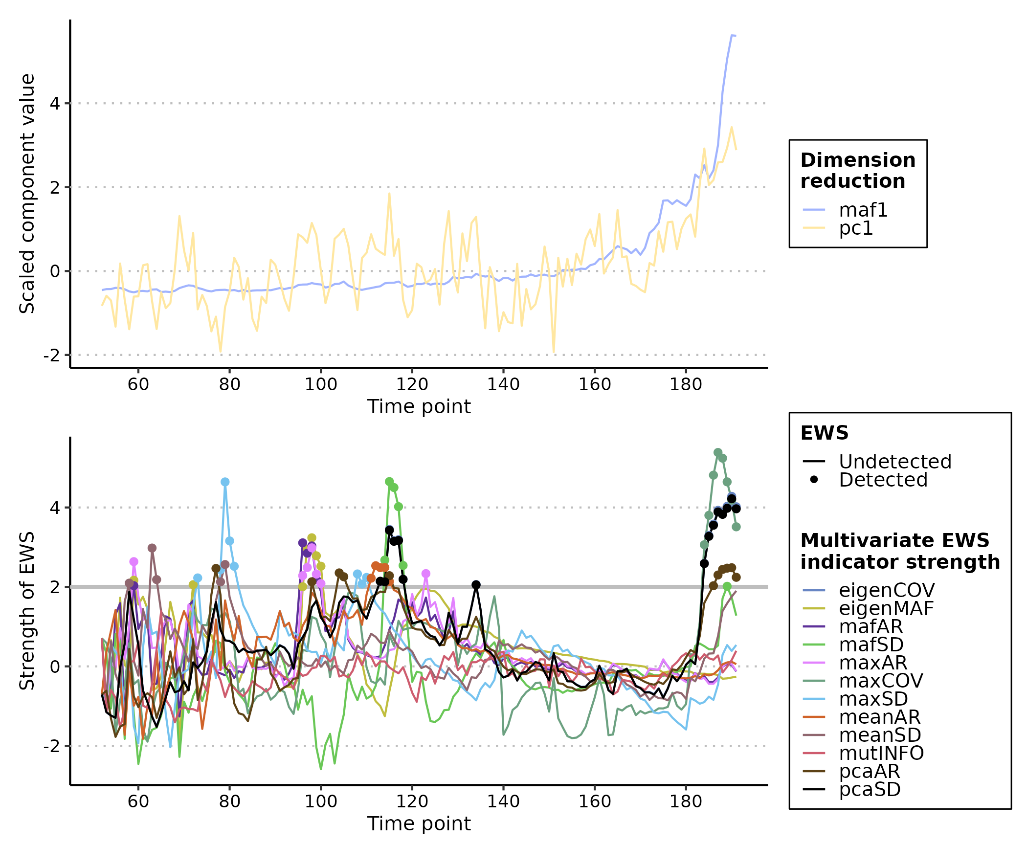

In this circumstance, many of the indicators are warning at different times (e.g. "eigenMAF" at time ~= 65 or "meanAR" at time ~= 100) but that the vast majority are warning in the last 20 time points. This highlights the usefulness of expanding windows over rolling as the exact time point of warning can be determined, and supports Weinans et al.’s (2021) suggestion that there is no superior multivariate EWS indicator; the best fit depends on the scenario the system is subject t0.

FAQ

1. How do I interpret EWSs?

Rolling windows

The simplicity of the rolling window approach also limits its usefulness. A ‘warning’ is indicated when an EWS displays a strong positive Kendall Tau correlation with time. However, it is unclear what constitutes a ‘strong’ correlation in this context with published warnings ranging from 0.5 through to 0.9 (Dakos et al. 2012, Dablander et al. 2022, Southall et al. 2022). The strength of correlation therefore appears to be context dependent and system specific.

An alternative approach suggested by Dakos et al. (2012) is to generate random permutations of the assessed time series and then compare the estimated Kendall Tau coefficients to that of the ‘true’ time series. If the true coefficient is stronger than 95% of the permuted coefficients then that represents a warning.

Expanding windows

Expanding windows have a stronger evidence base for what constitutes a ‘warning’. Clements et al. 2019 show that two consecutive transgressions of the 2σ threshold reduce false-postive rates and improve the number of true-postives. This has been validated by Southall et al. 2022 although they suggest that more than two consecutive signals should be aimed for.

2. Do I need to detrend my data?

The is a body of work that suggests detrending may be necessary to improve the reliability of early warning signal indicators (Dakos et al. 2012, Gama Dessavre et al. 2019, Lenton et al. 2012). EWSmethods therefore provides a simple detrending function detrend_ts() which provides four methods of detrending a time series:

Detrending method code	Description
linear	Linear detrending - returns the residuals of a fitted linear model between the time index and time series
loess	Local polynomial regression smoothing - subtracts a smooth curve fitted by local polynomial regression from the observed time series
gaussian	Gaussian kernel smoothing - subtracts a smooth curve estimated by a kernel based weighted moving average from the observed time series
first.difference	First differencing - subtracts the lagged time series from the unlagged time series

Example:

detrend_dat <- detrend_ts(data =  pre_simTransComms[,2:7],  method = "loess", span = 0.75, degree = 2)

matplot(x = detrend_dat$time, y = detrend_dat[,2:6], type = "l", xlab = "Date", ylab = "Density",  main = "LOESS detrended five species community")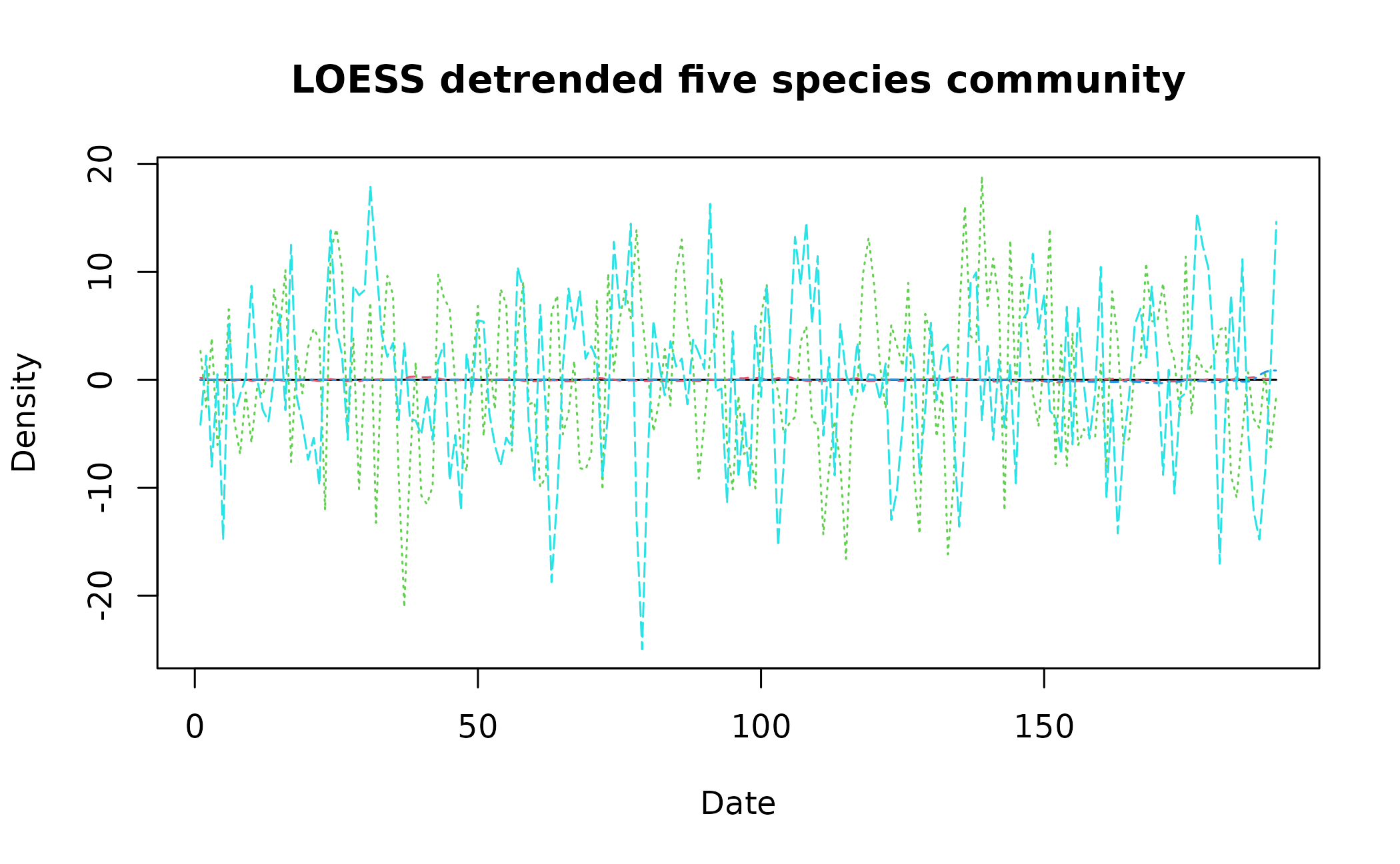

The current consensus is that detrending is required prior to univariate EWS analysis. However for non-average multivariate indicators, we suggest assessments should be made on non-detrended data as the trend is informative. Mutual information in particular suffers following detrending.

3. My data is seasonal/contains cycles. Can I still use Early Warning Signals?

Early warning signal indicators are particularly sensitive to cyclical data as the repeated non-linearity throughout the year/cycle period will be interpreted as a transition initially, before masking future cycles and tipping points. It is therefore sensible to deseason seasonal data prior to assessment.

EWSmethods provides a suite of average and time series decomposition deseasoning techniques via the deseason_ts() function. This function takes a n x m dataframe of time series to be deaseasoned. The first column must be a vector of dates with the increment = and order = arguments indicating the data resolution (year, month, day) and the order of the date vector (ymd/dmy/ydm). The form of deseasoning can then be selected using the method = argument.

Lets create some dummy monthly data that we can deseason.

spp_data <- matrix(nrow = 5*12, ncol = 5)

seasonal_cycle <-  20*sin(2*pi*(1:5*12)/12)

spp_data <- sapply(1:dim(spp_data)[2], function(x){

  spp_data[,x] <- ts(rnorm(5*12,mean = 20, sd = 3) + seasonal_cycle, freq = 12, start = c(2000, 1)) #add seasonal cycle to random noise
  
  })

multi_spp_data <- cbind("time" = base::seq(base::as.Date('2000/01/01'), base::as.Date('2004/12/01'), by = "month"), as.data.frame(spp_data))
  
matplot(x = multi_spp_data$time, y = multi_spp_data[,2:6], type = "l", xlab = "Date", ylab = "Density",  main = "Seasonal five species community")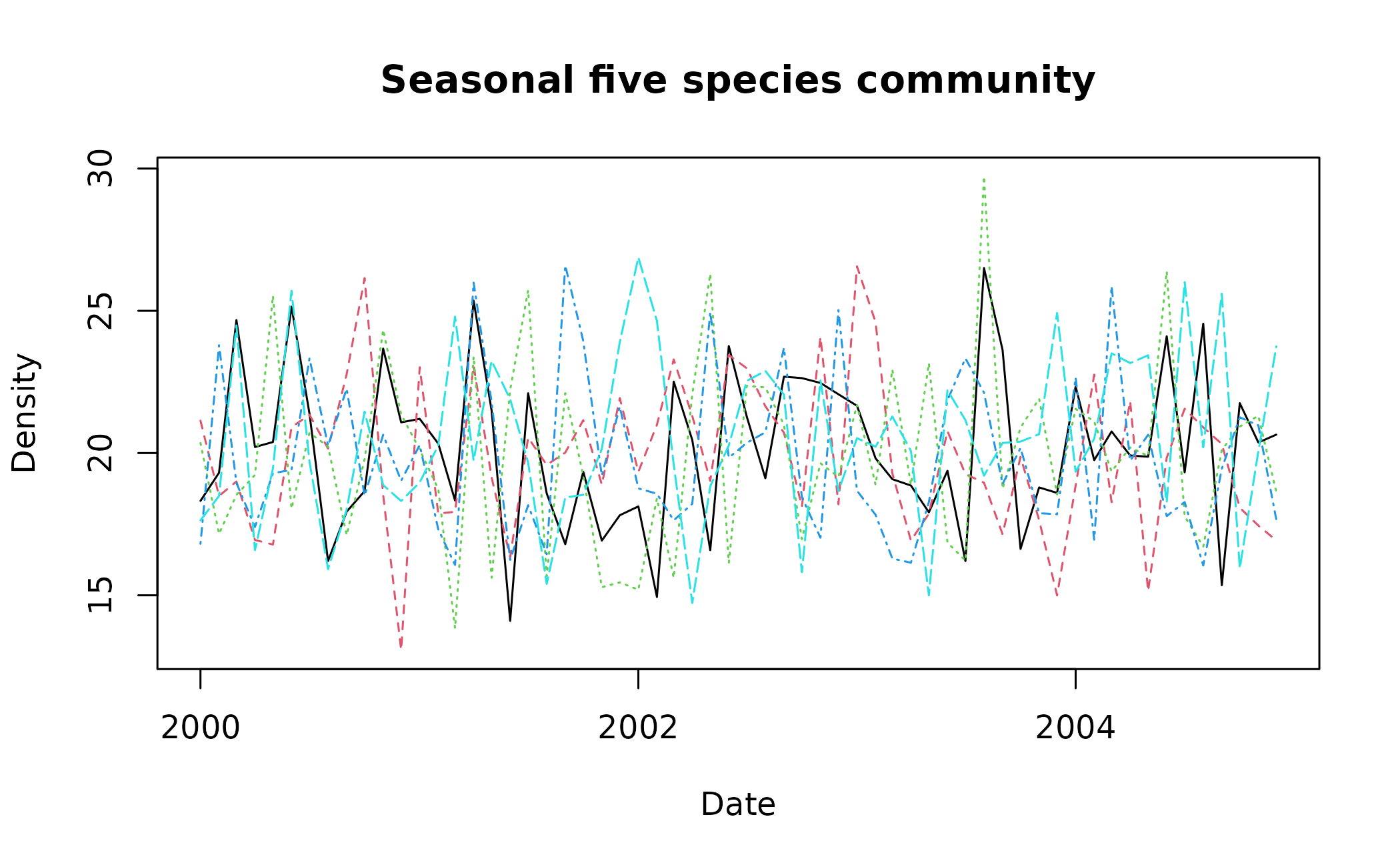

As multi_spp_data is random, there are few pronounced cycles but for the sake of this tutorial, deseason_ts() would be applied to it as such:

deseas_dat <- deseason_ts(data = multi_spp_data, increment = "month", method = "average", order = "ymd")
#> data successfully aggregated into monthly time steps

matplot(x = deseas_dat$date, y = deseas_dat[,2:6], type = "l", xlab = "Date", ylab = "Density",  main = "Deseasoned five species community")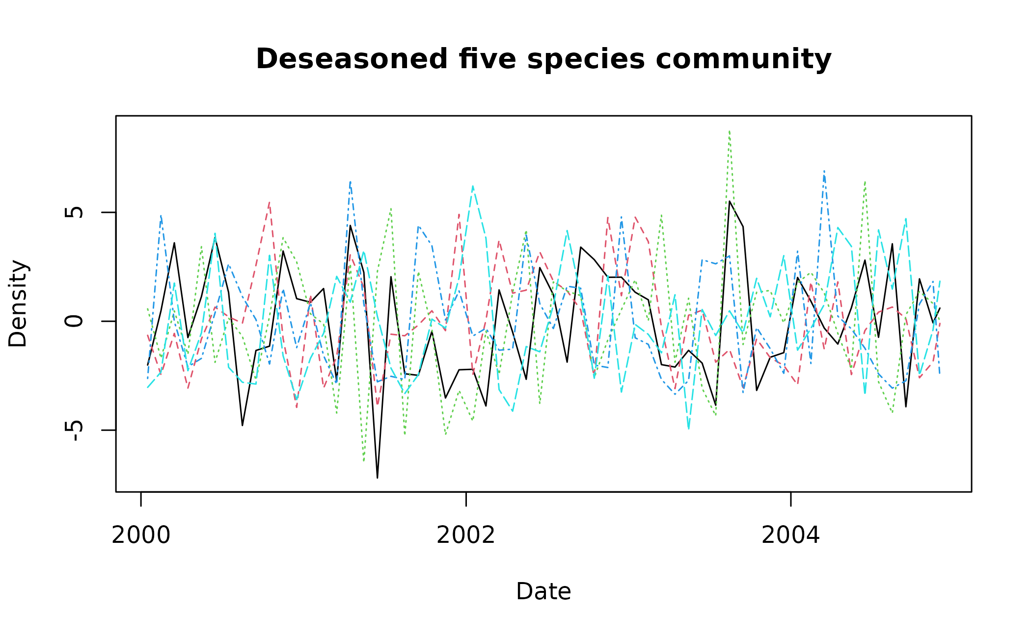

The method = "stl" argument shows that we have chosen to deseason using LOESS (locally weighted smoothing) by estimating the cyclical component for each time series and then subtracting it. method = "decompose" performs a similar process but uses classical decomposition. method = "average" is the simplest method where the average increment value is estimated for each unique increment and that value subtracted from each data point that shares that increment key. deseason_ts() simply provides the default procedure for each of these methods and consequently we visualise the results of deseason_ts() before using it in downstream analyses.

In our example, we can see that large monthly values shared across multiple years have been shrunk - e.g. the black dashed species at ~2001 - whereas anomalous values have been maintained - e.g. the green dotted species at ~2002.75.

References

Clements, C.F. & Ozgul, A. (2016) Including trait-based early warning signals helps predict population collapse. Nature Communications, 7, 10984. doi:10.1038/ncomms10984

Clements, C.F., McCarthy, M.A. & Blanchard, J.L. (2019) Early warning signals of recovery in complex systems. Nature Communications, 10, 1681. doi:10.1038/s41467-019-09684-y

Cleveland, R.B., Cleveland, W.S., McRae, J.E., & Terpenning, I.J. (1990) STL: A seasonal-trend decomposition procedure based on loess. Journal of Official Statistics, 6, 1, 3–33. http://bit.ly/stl1990

Dablander, F., Heesterbeek H., Borsboom D. & Drake J.M. (2022) Overlapping timescales obscure early warning signals of the second COVID-19 wave. Proceedings of the Royal Society B , 289, 20211809. doi:10.1098/rspb.2021.1809

Dakos, V. (2018) Identifying best-indicator species for abrupt transitions in multispecies communities. Ecological Indicators, 94, 494–502. doi:10.1016/j.ecolind.2017.10.024

Dakos, V., Carpenter, S.R., Brock, W.A., Ellison, A.M., Guttal, V., Ives, A.R., et al. (2012) Methods for detecting early warnings of critical transitions in time series illustrated using simulated ecological data. PLoS One, 7, e41010. doi:10.1371/journal.pone.0041010

Gama Dessavre, A., Southall, E., Tildesley, M.J. & Dyson, L. (2019) The problem of detrending when analysing potential indicators of disease elimination, Journal of Theoretical Biology, 481, 183-193. doi:10.1016/j.jtbi.2019.04.011

Ladiray, D., & Quenneville, B. (2001) Seasonal Adjustment with the X-11 Method. Springer. doi:10.1007/978-1-4613-0175-2

Lenton T M., Livina V.N., Dakos V., van Nes E.H. & Scheffer M. (2012) Early warning of climate tipping points from critical slowing down: comparing methods to improve robustness Philosophical Transactions of the Royal Society A 370, 1185–1204. doi:10.1098/rsta.2011.03047

O’Brien, D.A. & Clements, C.F. (2021) Early warning signal reliability varies with COVID-19 waves. Biology Letters, 17, 20210487. doi:10.1098/rsbl.2021.0487

Persons, W.M. (1919) General considerations and assumptions. The Review of Economics and Statistics, 1, 1,, 5–107. doi:10.2307/1928754

Southall E., Tildesley, M.J. & Dyson, L. (2022) How early can an upcoming critical transition be detected? medRxiv 2022.05.27.22275693. doi:10.1101/2022.05.27.22275693

Weinans, E., Quax, R., van Nes, E.H. & van de Leemput, I.A. (2021) Evaluating the performance of multivariate indicators of resilience loss. Scientific Reports, 11, 9148. doi:10.1038/s41598-021-87839-y