Using EWSNet

About this tutorial

This tutorial introduces how to interface with EWSNet, a machine learning model trained to predict critical transitions, tipping points, and regime shifts (Deb et al. 2022). We will only focus on how to set up your R session to interact with EWSNet and how to interpret the output rather than the theory and mathematics underlying the model. If you are interest in those details, please refer to the EWSNet specific website and documentation or the associated publication.

NOTE This version of EWSNet differs from that published by Deb et al. (2022) in that is has been retrained using a range of time series lengths (minimum = 15). This improves the accuracy of EWSNet over a range of time series lengths but we recommend that the minimum length to be tested should be 15 data points.

Getting started

set.seed(123) #to ensure reproducible data

library(EWSmethods)
library(ggplot2)
library(tidyr)

options(timeout = max(600, getOption("timeout"))) #due to possible internet issues, increase the timeout options from 60 seconds to 600

As EWSNet has been written and developed in Python, for R to interact with it, we need to exploit the reticulate R package. reticulate provides the tools to run Python code in R and transfer objects between the two languages but tends to run much smoother in RStudio rather than base R. It is therefore recommended that you use the RStudio IDE when using the EWSNet portion of EWSmethods.

The following sections will show how to setup and run EWSNet in EWSmethods before troubleshooting a few common errors stemming from the Python-reticulate-R interface.

1. Initialising EWSNet

Rather than requiring the user to learn reticulate and setup the R session themselves, EWSmethods provides a single function capable of checking your machine for Python, installing it if it’s not found (along with the critical packages), creating a new Python environment to hold these packages, and then activating that environment when ready. To prevent the user accidentally installing Python or packages, the function does require confirmation inputs from the user and so needs to be run at the start of any new R session.

For example, to create a new Python environment called "EWSNET_env" and install Python, the function would be written as below. The environment name ("EWSNET_env") will be critical to running the later functions.

#prepares your session using 'reticulate' and asks to install Anaconda (if no appropriate Python found) and/or a Python environment before activating that environment with the necessary Python packages
ewsnet_init(envname = "EWSNET_env", pip_ignore_installed = FALSE)

#> Error : Specified conda binary '/home/runner/.local/share/r-miniconda/bin/conda' does not exist.

If successful, you will have had to input "y" to allow EWSmethods to download and activate the Python environment and now see the message "EWSNET_env successfully found and activated. Necessary Python packages installed"). If not, please refer to the Troubleshooting section at the end of the tutorial.

To double check the environment activation, you could use reticulate functions to check first what environment is active and second what Python packages have been loaded:

library(reticulate)

#print which Python environment `EWSmethods` is using
reticulate::py_config()
#> python:         /home/runner/.local/share/r-miniconda/envs/test/bin/python
#> libpython:      /home/runner/.local/share/r-miniconda/envs/test/lib/libpython3.9.so
#> pythonhome:     /home/runner/.local/share/r-miniconda/envs/test:/home/runner/.local/share/r-miniconda/envs/test
#> version:        3.9.18 (main, Sep 11 2023, 13:41:44)  [GCC 11.2.0]
#> numpy:          /home/runner/.local/share/r-miniconda/envs/test/lib/python3.9/site-packages/numpy
#> numpy_version:  1.26.4
#> 
#> NOTE: Python version was forced by use_python() function

#list all packages currently loaded in to "EWSNET_env"
py_packages <- reticulate::py_list_packages() 
head(py_packages)
#>         package version       requirement   channel
#> 1 _libgcc_mutex     0.1 _libgcc_mutex=0.1 pkgs/main
#> 2 _openmp_mutex     5.1 _openmp_mutex=5.1 pkgs/main
#> 3       absl-py   2.1.0     absl-py=2.1.0      pypi
#> 4     alabaster  0.7.16  alabaster=0.7.16      pypi
#> 5    astunparse   1.6.3  astunparse=1.6.3      pypi
#> 6         babel  2.14.0      babel=2.14.0      pypi

EWSmethods also does not come bundled with the necessary model weights to make predictions. This is due the size of the weight files being ~220 MB which is not appropriate for all users of the package. To download these weights, we can use the ewsnet_reset() function which can either remove no-longer-needed weights or re/download from https://ewsnet.github.io.

ewsnet_reset(remove_weights = FALSE)

If successful, you will have had to input "y" to allow EWSmethods to download the pretrained weights.

2. Predictions from EWSNet

To give an example on how to use ewsnet_predict() we need some test data. Here, we will use some random noise around a mean of 0 which we expect to be predicted as "No Transition".

data("simTransComms")

pre_simTransComms <- subset(simTransComms$community1,time < inflection_pt)

plot(pre_simTransComms[,3], xlab = "Year", ylab = "Density")

We then simply provide this vector to ewsnet_predict() while also specifying the Python environment, the scaling of the data and ensemble number (how many models to average the prediction over).

ewsnet_prediction <- ewsnet_predict(pre_simTransComms[,3], scaling = TRUE, ensemble = 25, envname = "EWSNET_env") 

ewsnet_prediction
#> [1] "Call 'ewsnet_init()' before attempting to use ewsnet_predict(), or check your spelling of envname"

Interpreting EWSNet

As with any machine learning model, interpreting prediction probabilities is difficult. In EWSNet’s case, as three possible predictions can be made - No transition, Smooth transition, Critical transition - a chance prediction is one that is approximately 0.33 (1.0 divided by 3 is ~0.33).

Therefore any probability greater than 0.33 implies a stronger than chance prediction and anything greater than 0.6 warrants serious scrutiny.

Similarly, the real world manifestation of a Smooth or Critical transition is unclear (Kefi et al 2013, Gsell et al 2016). EWSNet therefore considers a "Smooth Transition" prediction to indicate a directional trend in the system whereas a "Critical Transition" indicates a rapid non-linear change. A "No Transition" prediction consequently suggests a stable period.

The below figure visually depicts the models that have been used to train these predictions and how those predictions relate to time series data.

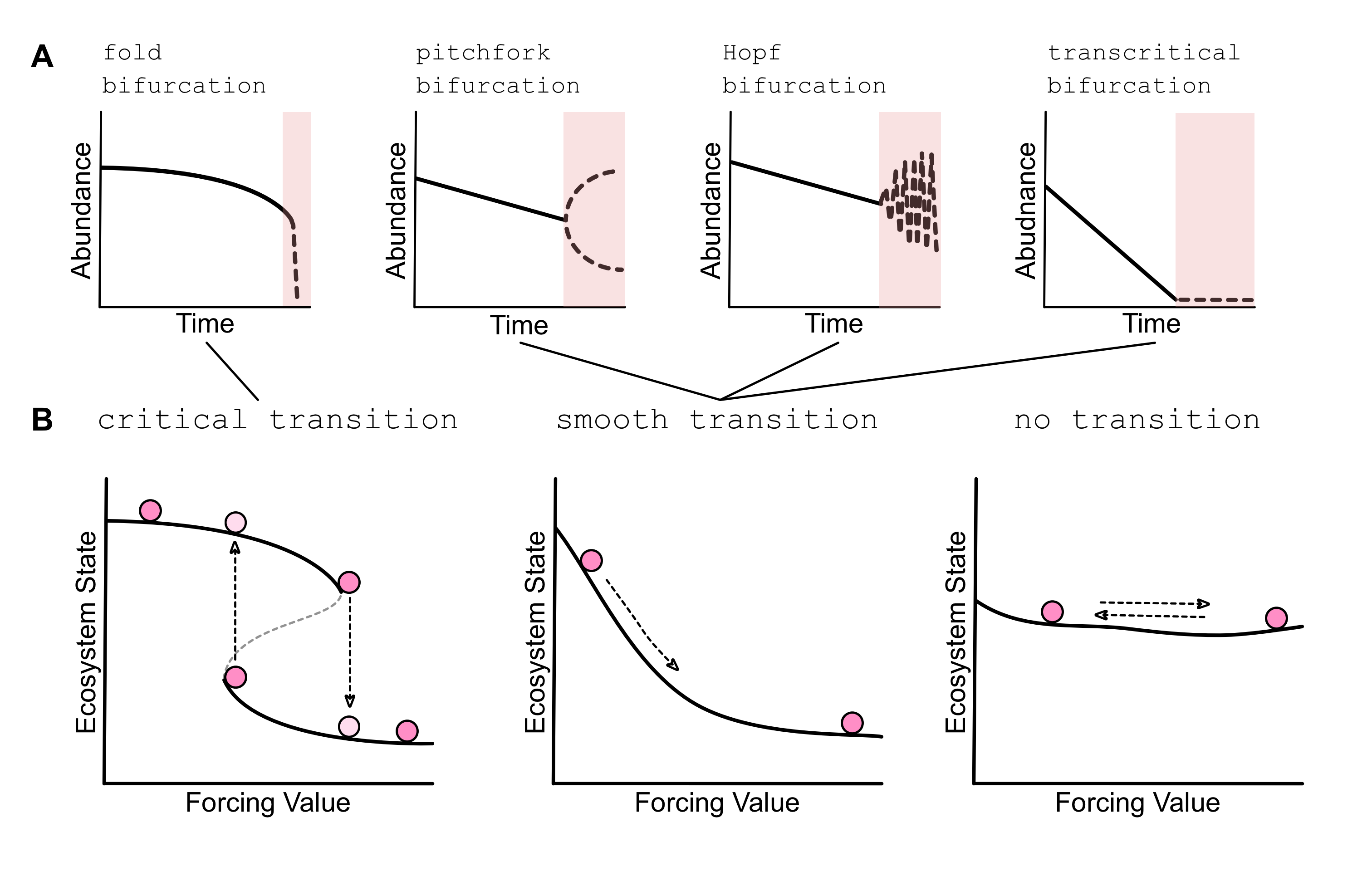
Conceptual diagram of A) the type of transitions that EWSNet has been trained on and B) how those transitons can appear in real time series data

Predictions through time

An additional way to use EWSNet is to explore how predictions change through time. By iteratively adding in new data, we can see how those predictions evolve.

For example, using our test data, we could use this code to identify transitions that may have happened in the past:


#define the range of indexes to test over
expanding_range <- 50:length(pre_simTransComms[,3]) 

#pre-define our out file
expanding_ewsnet <- data.frame(expanding_range, matrix(NA,ncol=3 )) |>
  `colnames<-`(c("cutoff_ind","No transition",'Smooth','Critical')) 

#call `ewsnet_predict()` for each index 
for(i in seq_along(expanding_range)){ 
  ews.tmp <- ewsnet_predict(pre_simTransComms[1:expanding_range[i],3],scaling = TRUE, ensemble = 25, envname = "EWSNET_env") 
  
  expanding_ewsnet[i,] <- c(expanding_range[i],ews.tmp$no_trans_prob,ews.tmp$smooth_trans_prob,ews.tmp$critical_trans_prob)
}

#plot the results
ggplot(expanding_ewsnet |> pivot_longer(-cutoff_ind,names_to = "Prediction",values_to = "prob"),
                aes(x=cutoff_ind,y=prob)) +
    geom_point(aes(col=Prediction)) + theme_bw() +
    xlab("Assessment index") + ylab("Prediction probability")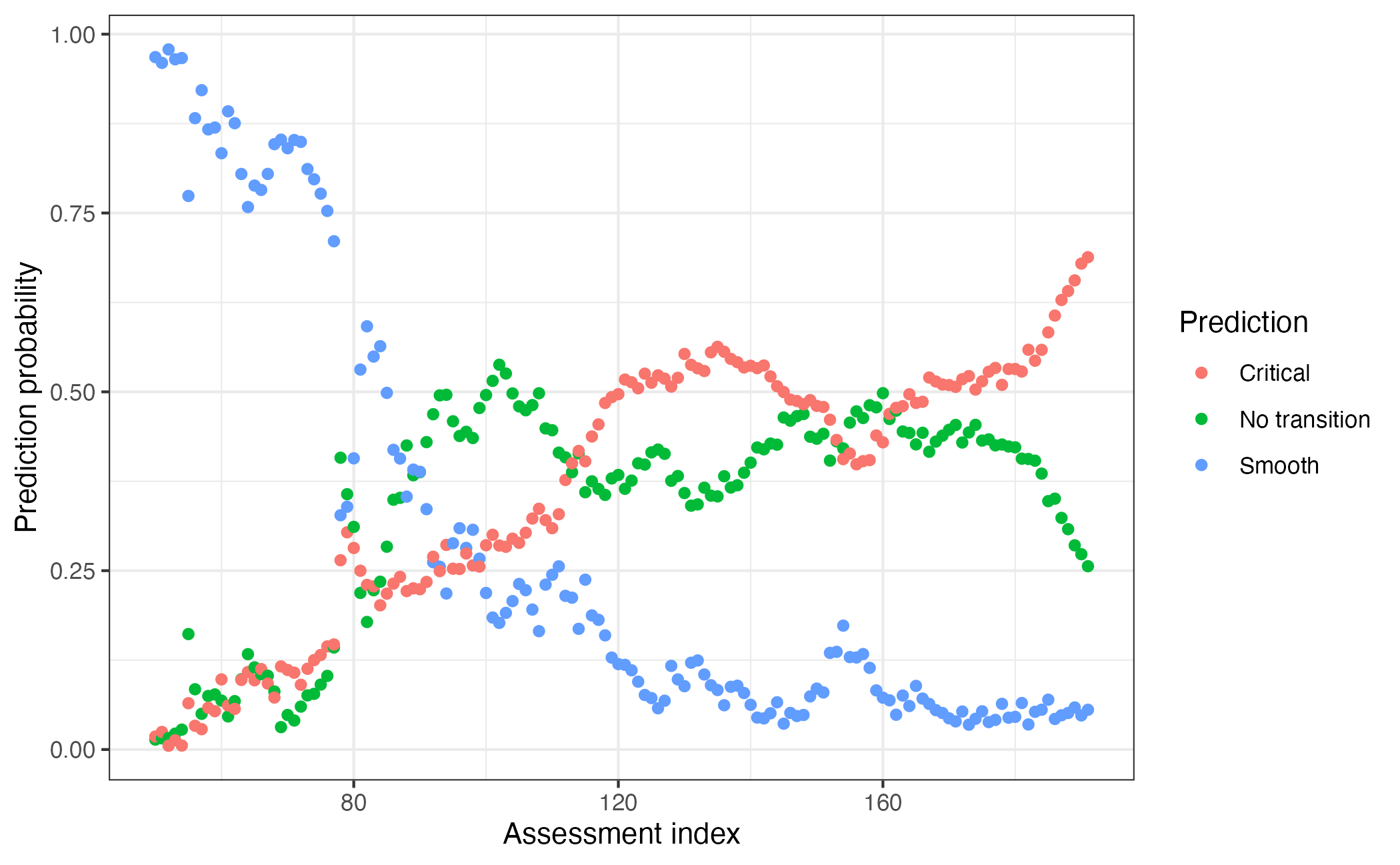

Here we see how prediction probabilities fluctuate with new data, with the trends in probabilities also providing information on how the system has changed over time.

3. Finetuning EWSNet

In the circumstance where training data is available, it may be preferable to finetune EWSNet. Finetuning alters the EWSNet model weights based upon the training data in an attempt to improve predictions. For example, the user could simulate their own collapsing time series of the same length as their test data. EWSNet would then be tuned to identify features specific to the time series of interest.

An example is given below using a mock data set matched to the same length of pre_simTransComms - 191 data points.

x <- matrix(nrow = length(pre_simTransComms[,3]), ncol = 10)

x <- sapply(1:dim(x)[2], function(i){
  x[,i] <- rnorm(length(pre_simTransComms[,3]),mean=20,sd=10)})
# create dummy data 

y <- sample(0:2,10,replace = TRUE)
# create labels. 0 = no transition, 1 = smooth transition, 2 = critical transition

ewsnet_finetune(x = x, y = y, scaling = TRUE, envname = "EWSNET_env")

Each of the 25 scaled model weights have resultingly been finetuned based upon the new training data. Calling ewsnet_predict(scaling = T) will therefore use these new weights.

In this example, as the training data has been randomly generated, the prediction quality will decrease, however it goes to show how weights can be updated/improved if new data comes available.

4. Resetting EWSNet

Following finetuning, it may be desirable to reset the model weights to their default. Using the ewsnet_reset() function, the user can direct EWSmethods to the path of the default weights (these can be redownloaded from the EWSNet github) which will overwrite the current model weights stored by EWSmethods.

ewsnet_reset(remove_weights = FALSE)

You may want to remove Python downloads and environment setup by EWSmethods and/or any downloaded EWSNet weights. You can achieve this using ewsnet_init() and the conda_refresh = argument, and ewsnet_reset() respectively.

conda_clean(envname = "EWSNET_env") # removes Python, its packages and the "EWSNET_env" environment

ewsnet_reset(remove_weights = TRUE) # removes any downloaded EWSNet weights

Quick reference

Function name	Purpose
`ewsnet_init()`	Prepares the session to interface with Python. Critical first step
`ewsnet_predict()`	Using the Python environment initialised by `ewsnet_init()`, builds the EWSNet model and makes predictions from the user supplied time series
`ewsnet_finetune()`	Retrains the initial EWSNet model weights based upon new user provided training data
`ewsnet_reset()`	Overwrites the model weights with the default weights downloaded from EWSNet github
`bypass_reticulate_autoinit()`	Optional set up function to get around quirks of`reticulate`
`conda_clean()`	Removes the Python installation and environment setup by `ewsnet_init()`

Greater detail on each function can be found at the Reference page.

Troubleshooting

1. `reticulate` is activating a different environment to the one I gave to `ewsnet_init()`

This is the main error when using EWSmethods. The first solution is to simply restart the R session and rerun ewsnet_init(). If reticulate is loaded before ewsnet_init() is run, then the default reticulate environment "r-reticulate" is activated instead of your EWSNet environment. Therefore ensure no reticulate command or library(reticulate) is run prior to ewsnet_init().

If the error remains and your RStudio version is >=1.4, you may need to edit your Python interpreter settings in RStudio’s preferences. Go to Preferences -> Python and untick “Automatically activate project-level Python environments”. Then restart your R session and rerun ewsnet_init().

The final solution we are aware of involves deactivating reticulate’s default behaviour in your global R environment settings. Running bypass_reticulate_autoinit() will disable reticulate’s ability to load a Python environment without a user request. Restart your R session and rerun ewsnet_init() once ready.

2. `ewsnet_predict()` is returning Python errors

These errors are extremely difficult to debug through R . Fortunately, in our experience, such errors are legacies of previous issues such as incorrect initialising of the Python environment, the crashing of an R session, or killing of the running function. The error is therefore often solved by restarting the R session and rerunning ewsnet_init().

If the error remains, please submit a bug report here.

3. I want to uninstall Python and its environments

conda_clean() provides the functionality to do this:

conda_clean(envname = "envname").

This function will remove any downloaded Python versions, packages or environments to allow a fresh install or permanent removal.

References

Deb S., Sidheekh S., Clements C.F., Krishnan N.C. & Dutta P.S. (2022) Machine learning methods trained on simple models can predict critical transitions in complex natural systems. Royal Society Open Science, 9, 211475. doi:10.1098/rsos.211475

Gsell AS, Scharfenberger U, Özkundakci D, Walters A, Hansson LA, Janssen AB, Nõges P, Reid PC, Schindler DE, Van Donk E, Dakos V & Adrian R. (2016) Evaluating early-warning indicators of critical transitions in natural aquatic ecosystems. PNAS, 113(50):E8089-E8095. doi:10.1073/pnas.1608242113

Kéfi S., Dakos V., Scheffer M., Van Nes E.H. & Rietkerk, M. (2013) Early warning signals also precede non-catastrophic transitions. Oikos, 122: 641-648. doi:10.1111/j.1600-0706.2012.20838.x

Duncan O’Brien

2024-03-18

About this tutorial

Getting started

1. Initialising EWSNet

2. Predictions from EWSNet

Interpreting EWSNet

Predictions through time

3. Finetuning EWSNet

4. Resetting EWSNet

Quick reference

Troubleshooting

1. `reticulate` is activating a different environment to the one I gave to `ewsnet_init()`

2. `ewsnet_predict()` is returning Python errors

3. I want to uninstall Python and its environments

References

Using EWSNet

Duncan O’Brien

2024-03-18

About this tutorial

Getting started

1. Initialising EWSNet

2. Predictions from EWSNet

Interpreting EWSNet

Predictions through time

3. Finetuning EWSNet

4. Resetting EWSNet

Quick reference

Troubleshooting

1. reticulate is activating a different environment to the one I gave to ewsnet_init()

2. ewsnet_predict() is returning Python errors

3. I want to uninstall Python and its environments

References

1. `reticulate` is activating a different environment to the one I gave to `ewsnet_init()`

2. `ewsnet_predict()` is returning Python errors