Alternative Stability Measures

About this tutorial

This tutorial introduces stability metrics distinct from critical slowing down based/Early Warning Signal indicators. The primary benefit of this collection of techniques is that they are both model and equilibrium free; they don’t assume a system is a equilibrium.

EWSmethods provides three distinct approaches to quantifying system stability. The tutorial will go through each in turn and give examples of their usage.

Greater detail on each function can be found at the Reference page.

Getting started

set.seed(123) #to ensure reproducible data

library(EWSmethods)
library(ggplot2) #for plotting

We will use the same multi-species community described in the Performing Early Warning Signal Assessments tutorial.

Briefly, the data object "simTransComms" contains three replicate datasets of a simulated five species community that has been driven to transition by the introduction of an invasive species (following Dakos 2018). The strength of impact by the invasive species gradually increases through time between t100 and t200 at which point it is held constant.

Lets load the data in:

data("simTransComms")

and plot one of the communities. The vertical dashed line represents a sudden transition due to the invasive species.

matplot(simTransComms$community1[,3:7], type = "l", xlab = "Time", ylab = "Density",  main = "Transitioning five species community")
abline(v=simTransComms$community1$inflection_pt,col = "grey60", lty = "dashed")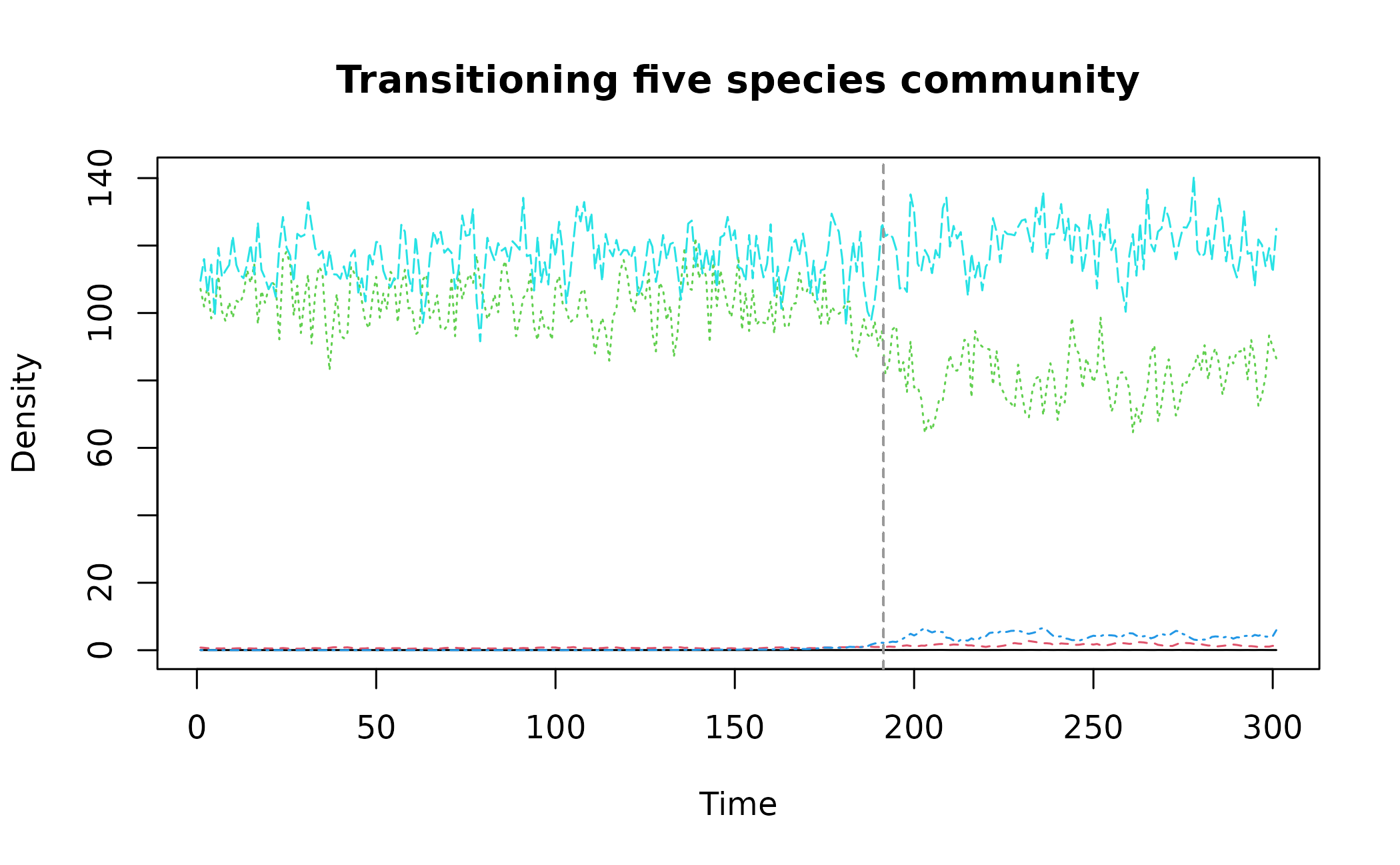

Now we have a system/community that is experiencing some form of stress and we can apply univariate or multivariate stability measures to give us an idea of how the system is responding to that stress.

1) Index of Variability

The simplest measure provided by EWSmethods is the multivariate index of variability (MVI - Brock and Carpenter, 2006). The MVI is represented by the square root of the dominant eigenvalue of the covariance matrix of all species.

Interpretation

Increasing MVI represents decreasing stability.

Usage

Provide the community data (first column being time, the remainder being species values) to the mvi() function, and specify a winsize to calculate the index over. The default winsize is 50% the total length of the time series, but we have set winsize = 25 to ensure that the periods before and after the sudden change in are distinct.

egMVI <- mvi(data = simTransComms$community1[,2:7], winsize = 25)

If we then plot the index, we can see that before and after the ‘inflection point’ (where the community goes through a transition) there are clear differences in stability.

What is also apparent is that the MVI begins to increase prior to the sudden change, albeit only slightly.

mvi_plot_data <- merge(simTransComms$community1,as.data.frame(egMVI),by="time") # combine the mvi data with the raw time series

ggplot(mvi_plot_data,aes(x = time, y = mvi)) + geom_line() + geom_vline(xintercept = mvi_plot_data$inflection_pt,col = "grey60", linetype = "dashed") + theme_bw() + xlab("Time") + ylab("MVI value")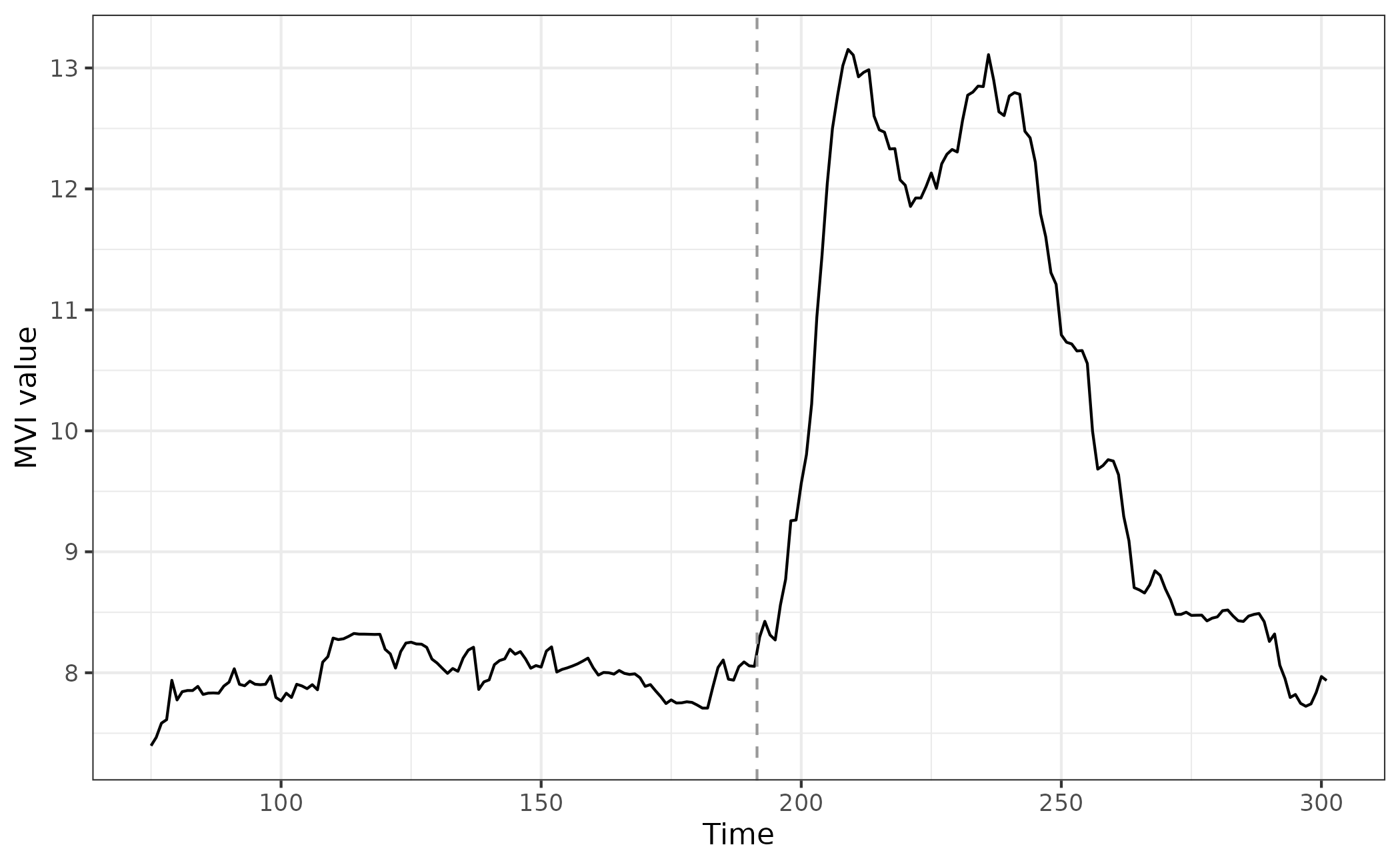

Caveats

The MVI only quantifies the variability of the community rather than changing relationships between community components. It is therefore susceptible to data quality, the inherent stochasticity of the system, and rate of forcing.

2) S-map Jacobians

The cutting edge of stability metrics belong to approaches which exploit empirical dynamic modelling (EDM - Sugihara et al. 2012). EDM exploits Takens’ embedding theorem (Takens 1981) which suggests that an underlying latent system/attractor manifold can be reconstructed from one or more related time series. By lag embedding two or more time series, their interaction strength (or causal strength) can be estimated.

This approach consequently requires no knowledge of the underlying equations nor numerical estimates of the system’s equilibrium state as the local Jacobians are directly estimated from the time series. The local Lyapunov stability is calculated as the dominant eigenvalue of the estimated Jacobian matrix.

Jacobians consist of the first-order partial derivatives for a multivariate function and are critical to resilience quantification. They are so important because they allow us to differentiate two or more functions with respect to two or more variables, something not achievable using standard derivation. Jacobian matrices therefore provide insight in to how each variable (or species) in a system’s master equation will change in the successive time step; if we know the true Jacobian, we know the future.

EWSmethods provides access to two forms of s-map estimated Jacobians, one for univariate data (following Grziwotz et al. 2023) and another for multivariate data (following Ushio et al. 2018).

Interpretation

A local Lyapunov stability value (the returned index value) of less than 1 indicates that the community tends to recover faster from perturbations, assuming the interspecific interaction strengths and self-regulation effects are constant. Therefore, 1 represents a threshold above which the system is unstable and below which the system is stable. However, any persistent increase in Jacobian index is of concern for stability loss.

Usage - Univariate

The univariate form of Jacobian estimated stability is performed using the uniJI() function. Following Grziwotz et al. (2023), uniJI() estimates the strength of time embedded relationship between a univariate time series and lagged forms of itself.

In uniJI(), we again provide community data but for a single species (first column being time, focal species the second). We must also provide a winsize, embedding dimension (E) and tau. E and tau are complicated to parameterise and requires a degree of exploration. Initially, we suggest E to be in the range 1 to 6, and tau in the range 3 - 12, but refer readers to the excellent introduction by Chang et al. (2017) for further details.

eg_uniJI <- uniJI(data = simTransComms$community1[,2:3], winsize = 25, E = 3)

Plotting the index for this species, we observe a loss of stability prior to the transition and dramatic overcompensation following it.

uniJI_plot_data <- merge(simTransComms$community1,eg_uniJI,by="time") # combine the mvi data with the raw time series

ggplot(uniJI_plot_data,aes(x = time, y = smap_J)) + geom_line() + geom_vline(xintercept = uniJI_plot_data$inflection_pt,col = "grey60", linetype = "dashed") + theme_bw() + xlab("Time") + ylab("Univariate stability index value")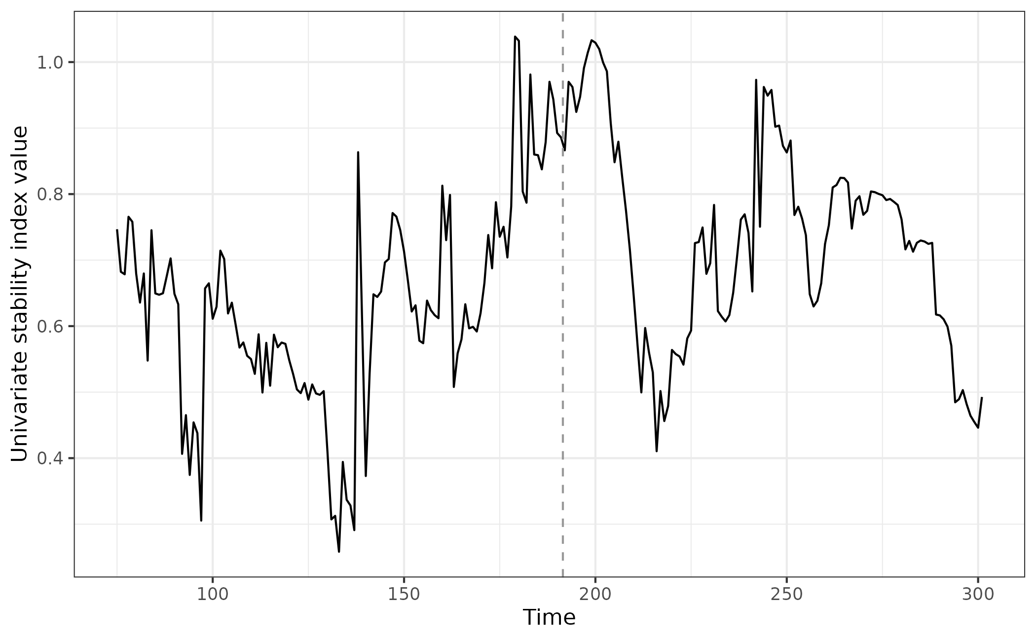

Lets repeat this for all species to give us an overall idea of system resilience.

all_spp_uniJI <- sapply(grep("spp_",colnames(simTransComms$community1)),FUN = function(x){
  if(x == 3){
  uniJI(data = simTransComms$community1[,c(2,x)], winsize = 25, E = 3)
  }else{
  uniJI(data = simTransComms$community1[,c(2,x)], winsize = 25, E = 3)[,2]
  }
  }) # for each species, calculate the univariate stability index

all_spp_uniJI <- do.call("cbind",all_spp_uniJI) # merge the list in to a data.frame
names(all_spp_uniJI) <- c("time",paste("spp",1:5,sep="_")) # and rename missing columns

all_spp_plot_data <- merge(tidyr::pivot_longer(all_spp_uniJI,cols = -time,names_to = "species",values_to = "smap_J"), simTransComms$community1[,c("time","inflection_pt")], by = "time") #pivot_longer for easier plotting and merge with the inflection point data

ggplot(all_spp_plot_data,aes(x = time, y = smap_J)) + geom_line(aes(col=species)) + geom_vline(xintercept = all_spp_plot_data$inflection_pt,col = "grey60", linetype = "dashed") + theme_bw() + xlab("Time") + ylab("Univariate stability index value") + scale_colour_manual(values = c("black","#6886c4","#bfbd3d","#69c756","#e281fe")) + facet_wrap(~species)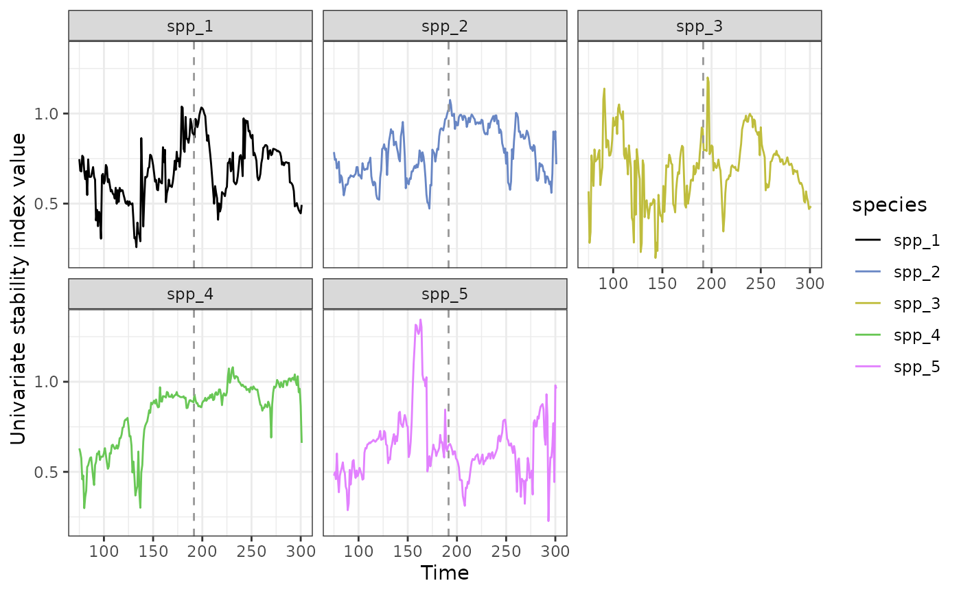

This approach highlights how each species responds uniquely and can help identify the most sensitive species. I.e which are possible indicator species.

Usage - Multivariate

Conversely, to compute the multivariate form of Jacobian estimation, we can use the function multiJI(). multiJI() fits a local linear model between all species which predicts the system’s future value from the reconstructed state-space. The resulting coefficients of this model are therefore a proxy for the interaction strength between species.

Note E and tau are not required for the multiJI() form of index. For E, the number of species themselves are used for embedding, though this does limit the minimum length of time series to being the number of species. Instead, theta is impactful, and represents the tuning parameter for forecasts (if not provided, multiJI() identifies the optimal theta using root mean square error). Conversely, tau is held constant at -1 as there is no self embedding due to the index being a multivariate measure.

⚠️ Warning! - multiJI() is significantly slower than any of the other resilience indicators provided by EWSMethods due to the multiple cross referencing required between species. Therefore increasing the number of species and length of time series (or decreasing winsize) can dramatically increase computation time.

eg_multiJI <- multiJI(data = simTransComms$community1[,2:7], winsize = 25)

Plotting the index for this species, we observe a loss of stability significantly prior to the transition and much earlier than the uniJI() estimated index.

multiJI_plot_data <- merge(simTransComms$community1,eg_multiJI,by="time") # combine the mvi data with the raw time series

ggplot(multiJI_plot_data,aes(x = time, y = smap_J)) + geom_line() + geom_vline(xintercept = multiJI_plot_data$inflection_pt,col = "grey60", linetype = "dashed") + theme_bw() + xlab("Time") + ylab("Mulivariate stability index value")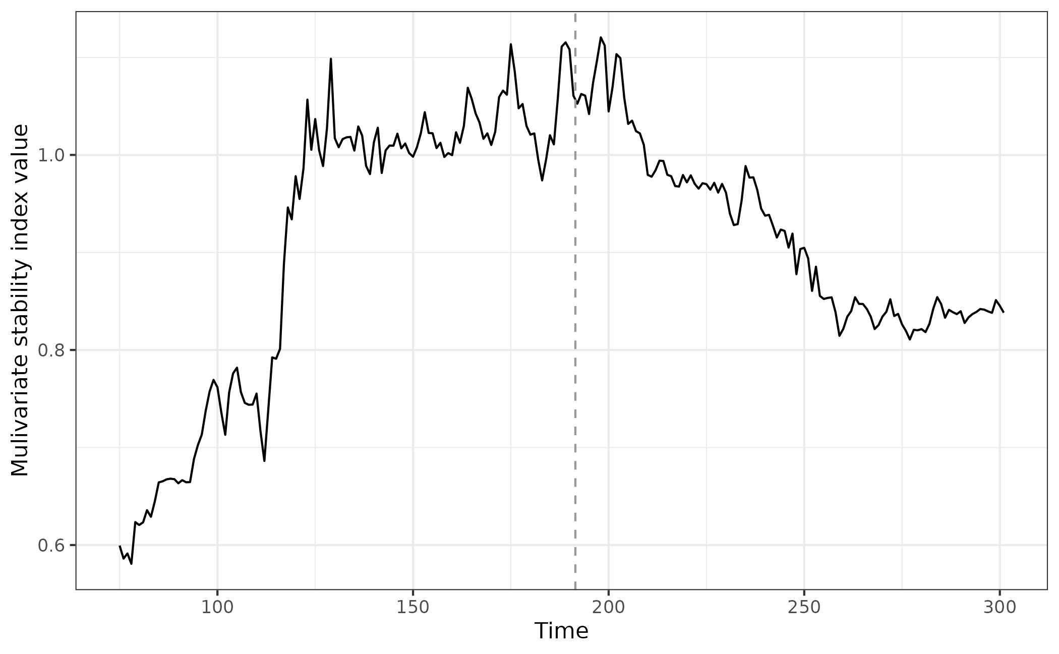

Caveats

Both s-map methods are sensitive to the choice of E and tau. Additionally, in seasonal/cyclical data, the shared cycles or seasons across species can artificially inflate estimates of causality and relatedness. In these circumstances, it is recommended to detrend data prior to estimating these stability metrics (Ushio et al. 2018). EWSmethods provides the capability to detrend and deaseason data via the functions detrend_ts() and deseason_ts() respectively. Similarly, it is sensible to scale/normalise all time series to be of equivalent magnitude to aid model fitting. A scale = TRUE argument is present in both uniJI() and multiJI() to achieve this.

Additionally, the two approaches require time series with no extended period of unchanging values (specifically a period equal to or longer than the window size). If uniJI() or multiJI() detect such a circumstance, the current iteration returns NA and the time series is removed respectively. For multiJI() if there are more species than data points in the window, then the index will fail. This is due to a multivariate index calculated across n species time delays up to lag n-1, which may not be possible if the time series are short. In this circumstance, we recommend sampling a subset of species, either randomly or the most abundance species (those less likely to have a period of unchanging values).

3) Autocorrelation Jacobians

An alternative method of estimating the Jacobian has been suggested by Williamson and Lenton (2015) which uses multivariate lag-1 autoregressive models rather than S-map reconstruction. In this approach, multivariate models estimate an autocorrelation matrix between all time series, the real eigenvalues of which are related to the real eigenvalues of the Jacobian:

\[\begin{equation} \lambda_{j}= \frac{1}{\Delta t}log \left| a_{j} \right| \end{equation}\]

where \(\lambda\) is the Jacobian eigenvalues, \(a_{j}\) is the eigenvalues of the autocorrelation matrix and \(\Delta t\) is the time step of the data generating process. As \(\Delta t\) is typically unknown for empirical data, we have assumed it is equal to 1, but this is an argument that can be altered.

Interpretation

As with multiJI, multiAR estimates local Lyapunov stability but with a threshold of 0 rather than 1. Consequently, we expect instability when multiAR > 0, stability when multiAR < 0, and for the value to trend positively with stress.

Usage

Lets estimate the index:

eg_multiAR <- multiAR(data = simTransComms$community1[,2:7], winsize = 25)

Plotting the index for this species, we observe very similar behaviour to multiJI(). This is encouraging as both indices estimate equivalent Jacobian matrices.

multiAR_plot_data <- merge(simTransComms$community1,eg_multiAR,by="time") # combine the mvi data with the raw time series

ggplot(multiAR_plot_data,aes(x = time, y = multiAR)) + geom_line() + geom_vline(xintercept = multiAR_plot_data$inflection_pt,col = "grey60", linetype = "dashed") + theme_bw() + xlab("Time") + ylab("Mulivariate stability index value")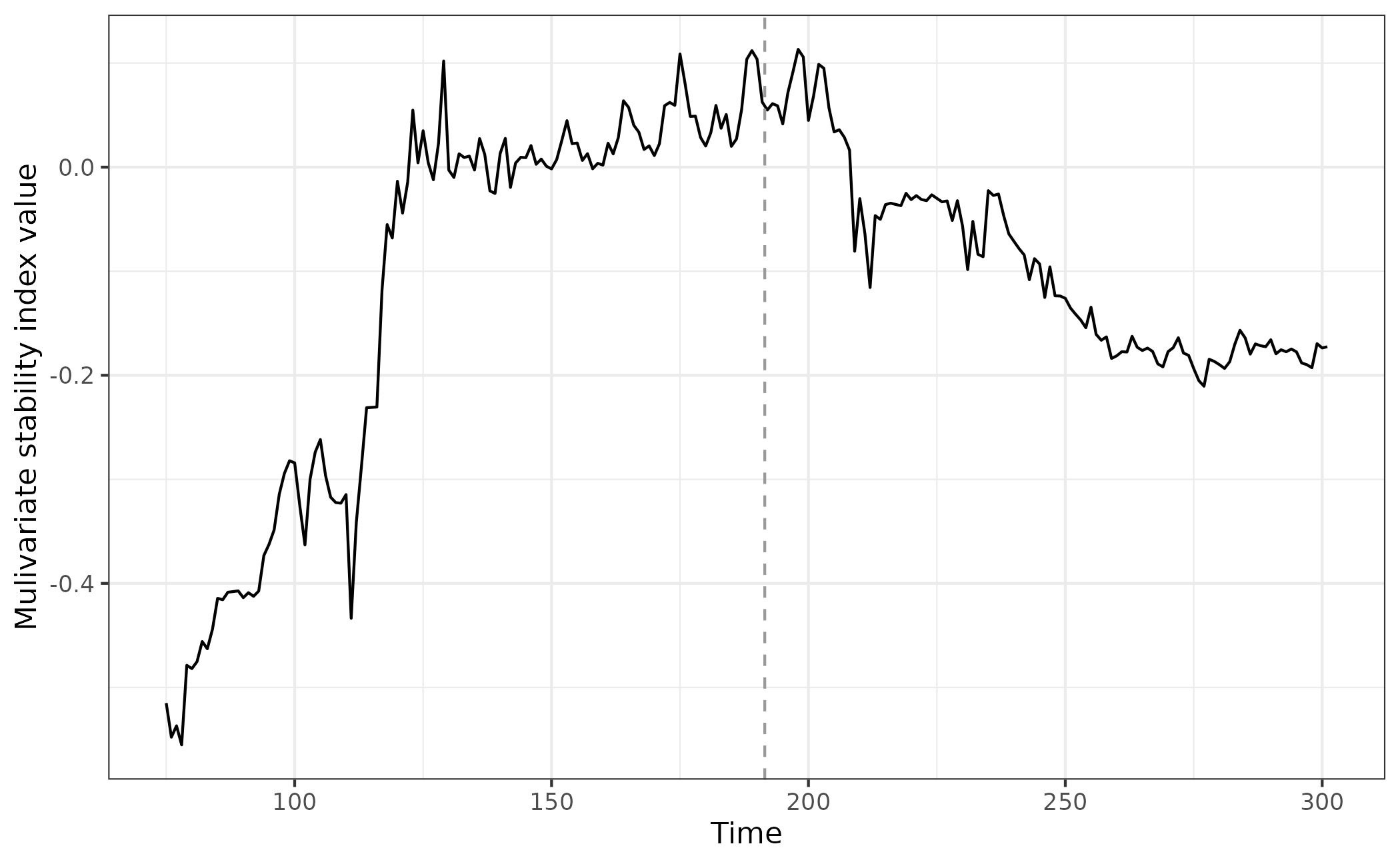

Caveats

multiAR suffers similar caveats to the S-map indices with a sensitivity to time series length and choice of time series contributing to the estimate. Anecdotally, the multivariate autoregressive models also require a minimum of 16 time points to function though the index estimation is ~25x faster than multiJI.

4) Fisher Information

Fisher Information (FI) attempts to estimate the amount of information data can provide on an unmeasured parameter (Fisher and Russell 1922). It consequently has been applied as an indicator of system dynamics and stability (Ahmad et al. 2016). EWSmethods provides a simplified discrete time form of Fisher and Russel (1922)’s mathematic proof following Karunanithi et al. (2008):

\[\begin{equation} FI\approx 4 \sum_{i=1}^{m}[q_i-q_{(i+1)}]^2 \end{equation}\]

where \(q_{i}^2\) is the amplitude of the probability of observing states of the system at time window \(i\) and \(m\) is the number of possible ‘states’. Possible states are defining by comparing the difference between temporally adjacent data windows to a reference ‘uncertainty’. If the absolute difference in density is less than the reference deviation for all variables (i.e. species densities), then the windows are binned in to the same ‘state’.

Interpretation

Decreasing FI represents decreasing stability.

Usage

Provide the community data (first column being time, the remainder being species values) to the FI() function, specify a winsize to calculate the index over, and a size-of-states vector (sost). The default winsize is 50% the total length of the time series, and sost is typically suggested to be the standard deviation of each species across the entire time series multiplied by 2 (Karunanithi et al. 2008). winspace indicates the number of data points to slide the rolling window along (1 is standard) and TL is the ‘tightening level’. TL is the percentage of points shared between states and allows the algorithm to classify data points to/from the same state.

eg.sost <- t(apply(simTransComms$community1[,3:7], MARGIN = 2, FUN = sd)) # define size-of-states using the standard deviation of each species separately. Must be wide format hence t()

egFI <- FI(data = simTransComms$community1[,2:7], sost =  eg.sost, winsize = 25,winspace = 1, TL = 90)$FI

If we again plot the index, we can see that before and after the ‘inflection point’ (where the community goes through a transition) there are clear differences in stability.

What is also apparent, is that the FI begins to decrease prior to the sudden change, and stability only returns after an extended period post constant stress (stress is constant from t200 onward).

fi_plot_data <- merge(simTransComms$community1,egFI,by="time") # combine the mvi data with the raw time series

ggplot(fi_plot_data,aes(x = time, y = FI)) + geom_line() + geom_vline(xintercept = fi_plot_data$inflection_pt,col = "grey60", linetype = "dashed") + theme_bw() + xlab("Time") + ylab("Fisher Information value")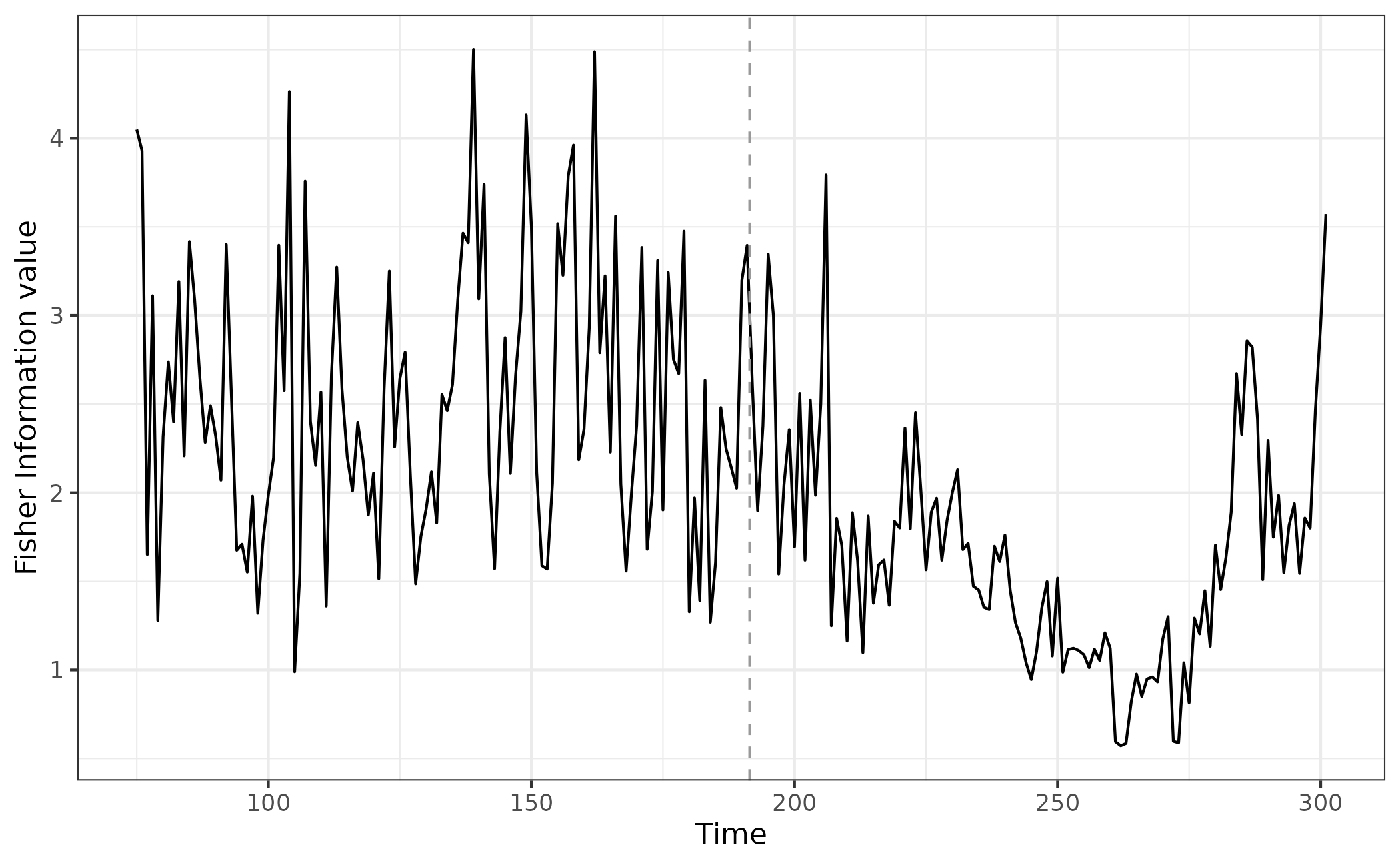

Caveats

FI is very sensitive to the size-of-states and tightening level. There is also no threshold of stable vs unstable as it is the relative change of FI that is important, not the absolute value.

References

Ahmad N., Derrible S., Eason T., and Cabezas H. (2016) Using Fisher information to track stability in multivariate systems. Royal Society Open Science. 3, 11, 160582. doi: 10.1098/rsos.160582

Brock, W., & Carpenter, S. (2006). Variance as a leading indicator of regime shift in ecosystem services. Ecology and Society, 11, 9. http://www.ecologyandsociety.org/vol11/iss2/art9/

Chang, C.-W., Ushio, M., and Hsieh, C.-h. (2017). Empirical Dynamic Modeling for beginners. Ecological Research, 32,6,785–796. doi:10.1007/s11284-017-1469-9

Fisher, R. A., & Russell, E. J. (1922). On the mathematical foundations of theoretical statistics. Philosophical Transactions of the Royal Society of London Series A: Containing Papers of a Mathematical or Physical Character, 222, 309–368. doi:10.1098/rsta.1922.0009

Grziwotz, F., Chang, C.-W., Dakos, V., et al. (2023). Anticipating the occurrence and type of critical transitions. Science Advances, 9. doi:10.1126/sciadv.abq4558

Karunanithi, A. T., Cabezas, H., Frieden, et al. (2008). Detection and assessment of ecosystem regime shifts from Fisher Information. Ecology and Society, 13, 1. https://www.jstor.org/stable/26267924

Sugihara, G., May, R., Ye, H., Hsieh, C., Deyle, E., Fogarty, M., & Munch, S. (2012). Detecting causality in complex ecosystems. Science, 338, 496–500. doi:10.1126/science.1227079

Takens, F. (1981). Detecting strange attractors in turbulence. Dynamical Systems and Turbulence, Warwick 1980. Ed. by D. Rand and L.-S. Young. Berlin, Heidelberg: Springer Berlin Heidelberg, pp. 366–381

Ushio, M., Hsieh, Ch., Masuda, R. et al. (2018) Fluctuating interaction network and time-varying stability of a natural fish community. Nature, 554, 360–363. doi:10.1038/nature25504

Williamson and Lenton (2015). Detection of bifurcations in noisy coupled systems from multiple time series. Chaos, 25, 036407. doi:10.1063/1.4908603

Duncan O’Brien

2024-03-18

About this tutorial

Getting started

1) Index of Variability

Interpretation

Usage

Caveats

2) S-map Jacobians

Interpretation

Usage - Univariate

Usage - Multivariate

Caveats

3) Autocorrelation Jacobians

Interpretation

Usage

Caveats

4) Fisher Information

Interpretation

Usage

Caveats

References